Analyzing and monitoring floods using Python and Sentinel-2 satellite imagery on NSIS Cloud
Comparing satellite observations before and during a flood can reveal changes in surface water, provided that both observations cover the same area and contain usable pixels. This worked example uses Sentinel-2 L2A observations around Wrocław from 6 and 21 September 2024.
Prerequisites
No. 1 Downloaded Sentinel-2 products
Start with the two Sentinel-2 products already downloaded and extracted. Prepare them by following Downloading Polish Sentinel-2 data with curl and wget on NSIS Cloud. For the general authentication and download procedure, see Using curl and wget to download EODATA products from NSIS Cloud.
Both extracted .SAFE directories must be directly inside ~/wroclaw-tutorial/data. Keep their complete contents and original names. This article starts from these local files.
The study area is 16.7–17.2° E and 50.9–51.4° N. The observations share tile T33UXS and relative orbit R122:
Role |
Acquisition |
Satellite / level |
Catalogue identifier |
|---|---|---|---|
Before the event |
6 September 2024 |
Sentinel-2B L2A |
3ef54189-a223-43fd-ab03-13010274a96b |
During the event |
21 September 2024 |
Sentinel-2A L2A |
e0d748d9-6190-46a7-b9e2-a1c898e5a686 |
These names identify the two Sentinel-2 products listed in the table. Each .SAFE directory contains product metadata, image-band files and scene-classification data. Keep the complete directory structure intact so the script can find the required files.
S2B_MSIL2A_20240906T095549_N0511_R122_T33UXS_20240906T160538.SAFE
S2A_MSIL2A_20240921T100031_N0511_R122_T33UXS_20240921T123352.SAFE
In your Bash terminal, list the contents of the data directory:
cd "$HOME/wroclaw-tutorial"
ls data
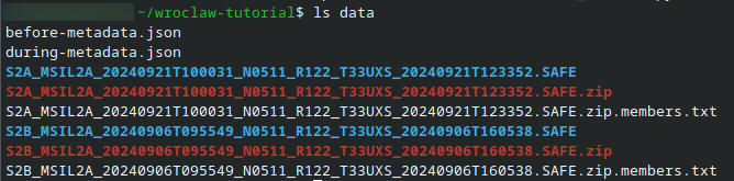
The two .SAFE directories shown here are the required inputs. ZIP archives and JSON files may also be present.
Confirm that both .SAFE directories are present before continuing. ZIP archives alone are not ready for the processing script; complete extraction using the download article first.
Both products were downloaded with authentication and then processed. The figures were generated from these actual scenes and reviewed alongside the study-area masks. The map shows possible areas of new surface water. Further checks against independent flood maps or field observations are needed to confirm which areas were flooded.
No. 2 Python environment and storage
Run the terminal commands in Bash. Copy each command block into the terminal and press Enter.
On Ubuntu, install Python 3 and venv support. Installing these system packages requires sudo privileges:
sudo apt update
sudo apt install python3 python3-venv
Use ~/wroclaw-tutorial as the working directory. Create and activate the Python virtual environment there:
mkdir -p "$HOME/wroclaw-tutorial"
cd "$HOME/wroclaw-tutorial"
python3 -m venv .venv
source .venv/bin/activate
Install the Python libraries in the active virtual environment:
python3 -m pip install numpy rasterio matplotlib
Allow space for both extracted .SAFE directories and the output files. Keep scripts and results in ~/wroclaw-tutorial, with the input products in the data subdirectory.
No. 3 Processing script
Save flood_wroclaw.py in ~/wroclaw-tutorial. You can download the file or copy the Python listing from this article into the file named in its first comment. Save the file before running the processing command in Step 1. Run all subsequent commands from the working directory with the virtual environment active. The python3 command then runs the interpreter installed in that environment.
Step 1: Run the processing script
The script compares the same area in both images and saves maps of the changes. It reads the products from ./data and writes the results to a new wroclaw-results subdirectory.
Save flood_wroclaw.py in ~/wroclaw-tutorial. Click the flood_wroclaw.py row to read or copy the code.
flood_wroclaw.py
# flood_wroclaw.py
"""Compare the specified Wroclaw L2A scenes on one calibrated 20 m grid.

Run only after obtaining the complete SAFE products. Outputs are candidate
surface-water changes; inspect RGB/SCL and event evidence before interpretation.
"""
import argparse
import json
import math
from pathlib import Path
import xml.etree.ElementTree as ET

import matplotlib
matplotlib.use('Agg')
import matplotlib.pyplot as plt
from matplotlib.colors import BoundaryNorm, ListedColormap
import numpy as np
import rasterio
from rasterio.transform import array_bounds
from rasterio.warp import reproject, Resampling, transform_bounds
from rasterio.windows import Window, from_bounds, transform as window_transform

PRODUCTS = {
    'before': ('2024/09/06', 'S2B_MSIL2A_20240906T095549_N0511_R122_T33UXS_20240906T160538.SAFE'),
    'during': ('2024/09/21', 'S2A_MSIL2A_20240921T100031_N0511_R122_T33UXS_20240921T123352.SAFE'),
}
AOI = (16.7, 50.9, 17.2, 51.4)  # west, south, east, north in EPSG:4326
BAND_IDS = {'B02': '1', 'B03': '2', 'B04': '3', 'B11': '11'}
VALID_SCL = (4, 5, 6)  # vegetation, non-vegetated land, water


def locate_safe(root, date, name):
    candidates = [root / name, root / 'Sentinel-2/MSI/L2A' / date / name]
    for path in candidates:
        if (path / 'MTD_MSIL2A.xml').is_file():
            return path
    raise FileNotFoundError(f'Complete SAFE product not found: {name}. Place it under --data-root, or use the mounted EODATA root.')


def band_path(safe, band):
    matches = sorted(safe.glob(f'GRANULE/*/IMG_DATA/R20m/*_{band}_20m.jp2'))
    if len(matches) != 1:
        raise ValueError(f'Expected one {band} 20 m file in {safe.name}; found {len(matches)}.')
    return matches[0]


def calibration(safe):
    root = ET.parse(safe / 'MTD_MSIL2A.xml').getroot()
    for node in root.iter():
        node.tag = node.tag.rsplit('}', 1)[-1]
    value = root.find('.//BOA_QUANTIFICATION_VALUE')
    if value is None or float(value.text) <= 0:
        raise ValueError('BOA_QUANTIFICATION_VALUE is missing or invalid.')
    offsets = {node.attrib['band_id']: float(node.text)
               for node in root.findall('.//BOA_ADD_OFFSET')}
    if not all(index in offsets for index in BAND_IDS.values()):
        raise ValueError('Expected L2A per-band BOA_ADD_OFFSET metadata; do not guess calibration.')
    return float(value.text), {band: offsets[index] for band, index in BAND_IDS.items()}


def common_grid(reference):
    with rasterio.open(reference) as src:
        if src.crs is None or not src.crs.is_projected:
            raise ValueError('Expected a projected Sentinel-2 grid.')
        if not np.allclose(src.res, (20, 20)):
            raise ValueError('Expected the L2A 20 m reference band.')
        bounds = transform_bounds('EPSG:4326', src.crs, *AOI, densify_pts=21)
        raw = from_bounds(*bounds, src.transform)
        left, top = math.floor(raw.col_off), math.floor(raw.row_off)
        right, bottom = math.ceil(raw.col_off + raw.width), math.ceil(raw.row_off + raw.height)
        if left < 0 or top < 0 or right > src.width or bottom > src.height:
            raise ValueError('The study area is not fully covered by the reference tile.')
        window = Window(left, top, right-left, bottom-top)
        return src.crs, window_transform(window, src.transform), (bottom-top, right-left)


def aligned(path, grid, categorical=False):
    crs, transform, shape = grid
    destination = np.full(shape, 0 if categorical else np.nan,
                          dtype=np.uint8 if categorical else np.float32)
    with rasterio.open(path) as src:
        reproject(source=rasterio.band(src, 1), destination=destination,
                  dst_transform=transform, dst_crs=crs, src_nodata=0,
                  dst_nodata=0 if categorical else np.nan,
                  resampling=Resampling.nearest if categorical else Resampling.bilinear)
    return destination


def calculate_mndwi(green, swir, scl):
    denominator = green + swir
    valid = np.isin(scl, VALID_SCL) & np.isfinite(green) & np.isfinite(swir)
    valid &= np.abs(denominator) > 1e-6
    result = np.full(green.shape, np.nan, dtype=np.float32)
    np.divide(green - swir, denominator, out=result, where=valid)
    return result


def compare(before, during):
    valid = np.isfinite(before) & np.isfinite(during)
    if not valid.any():
        raise ValueError('No jointly valid pixels. Inspect the scene masks and choose another pair.')
    difference = np.where(valid, during-before, np.nan)
    increase = np.where(valid, np.maximum(difference, 0), np.nan)
    new_water = np.where(valid, ((before <= 0) & (during > 0)).astype(np.uint8), 255).astype(np.uint8)
    return valid, difference, increase, new_water


def write_tif(path, array, grid, nodata=np.nan):
    crs, transform, shape = grid
    with rasterio.open(path, 'w', driver='GTiff', height=shape[0], width=shape[1],
                       count=1, dtype=array.dtype, crs=crs, transform=transform,
                       nodata=nodata, compress='deflate') as dst:
        dst.write(array, 1)


def plot_outputs(output, scenes, grid, difference, new_water):
    crs, transform, shape = grid
    west, south, east, north = array_bounds(*shape, transform)
    extent = (west, east, south, north)
    scl_cmap = ListedColormap(['black', 'red', '#444444', '#775533', '#228833',
                              '#ccbb66', '#3366cc', '#aaaaaa', '#cccccc',
                              'white', '#88ddff', '#ff99ff'])
    fig, axes = plt.subplots(2, 3, figsize=(15, 10), constrained_layout=True)
    for row, (label, scene) in enumerate(scenes.items()):
        rgb = np.stack([scene[band] for band in ('B04','B03','B02')], axis=-1)
        # The same fixed reflectance stretch is used for both dates.
        axes[row,0].imshow(np.clip(np.nan_to_num(rgb)/0.3, 0, 1), extent=extent)
        axes[row,0].set_title(f'{label}: RGB (reflectance 0–0.3)')
        image = axes[row,1].imshow(scene['SCL'], cmap=scl_cmap,
                                   norm=BoundaryNorm(np.arange(-.5,12.5),12), extent=extent, interpolation='nearest')
        fig.colorbar(image, ax=axes[row,1], ticks=range(12), label='SCL class')
        axes[row,1].set_title(f'{label}: scene classification')
        image = axes[row,2].imshow(scene['MNDWI'], vmin=-1, vmax=1, cmap='BrBG', extent=extent)
        fig.colorbar(image, ax=axes[row,2], label='MNDWI')
        axes[row,2].set_title(f'{label}: calibrated MNDWI')
    for ax in axes.flat:
        ax.set_xlabel(f'Easting (m), {crs.to_string()}'); ax.set_ylabel('Northing (m)')
    fig.savefig(output/'wroclaw_scene_review.png', dpi=160); plt.close(fig)
    fig, axes = plt.subplots(1,2,figsize=(12,6),constrained_layout=True)
    image = axes[0].imshow(difference, vmin=-1, vmax=1, cmap='RdBu', extent=extent)
    fig.colorbar(image,ax=axes[0],label='MNDWI during − before')
    axes[0].set_title('Change on jointly valid pixels')
    image = axes[1].imshow(np.ma.masked_equal(new_water,255), vmin=0,vmax=1,
                           cmap=ListedColormap(['#eeeeee','#2255aa']),extent=extent,interpolation='nearest')
    fig.colorbar(image,ax=axes[1],ticks=[0,1],label='Candidate new water')
    axes[1].set_title('Before ≤ 0 and during > 0 (MNDWI)')
    for ax in axes:
        ax.set_xlabel(f'Easting (m), {crs.to_string()}'); ax.set_ylabel('Northing (m)')
    fig.savefig(output/'wroclaw_water_change.png',dpi=160);plt.close(fig)


def main():
    parser = argparse.ArgumentParser(description=__doc__)
    parser.add_argument('--data-root', type=Path, required=True)
    parser.add_argument('--output', type=Path, default=Path('wroclaw-results'))
    args=parser.parse_args()
    if args.output.exists():
        raise FileExistsError('Choose a new output directory to preserve previous results.')
    safes={label:locate_safe(args.data_root,*values) for label,values in PRODUCTS.items()}
    grid=common_grid(band_path(safes['before'],'B11'))
    scenes={}
    report={'products':{label:path.name for label,path in safes.items()},
            'aoi_epsg4326':AOI,'crs':grid[0].to_string(),
            'shape':grid[2],'transform':list(grid[1])[:6],
            'valid_scl_classes':VALID_SCL,'water_threshold':0,'scenes':{}}
    for label,safe in safes.items():
        quant,offsets=calibration(safe)
        scene={band:(aligned(band_path(safe,band),grid)+offsets[band])/quant for band in BAND_IDS}
        scene['SCL']=aligned(band_path(safe,'SCL'),grid,categorical=True)
        scene['MNDWI']=calculate_mndwi(scene['B03'],scene['B11'],scene['SCL'])
        scenes[label]=scene
        values,counts=np.unique(scene['SCL'],return_counts=True)
        report['scenes'][label]={'quantification_value':quant,'offsets':offsets,
                                 'scl_pixel_counts':dict(zip(map(str,values),map(int,counts))),
                                 'valid_fraction':float(np.isfinite(scene['MNDWI']).mean())}
    valid,difference,increase,new_water=compare(scenes['before']['MNDWI'],scenes['during']['MNDWI'])
    pixel_area=abs(grid[1].a*grid[1].e-grid[1].b*grid[1].d)
    report.update(jointly_valid_fraction=float(valid.mean()),
                  candidate_new_water_hectares=float(np.sum(new_water==1)*pixel_area/10000),
                  interpretation='Unvalidated candidate surface-water change; requires RGB/SCL and event review.')
    args.output.mkdir(parents=True)
    for label,scene in scenes.items():
        write_tif(args.output/f'mndwi_{label}_wroclaw.tif',scene['MNDWI'],grid)
        write_tif(args.output/f'scl_{label}_wroclaw.tif',scene['SCL'],grid,nodata=0)
    write_tif(args.output/'mndwi_difference_wroclaw.tif',difference,grid)
    write_tif(args.output/'positive_change_wroclaw.tif',increase,grid)
    write_tif(args.output/'candidate_new_water_wroclaw.tif',new_water,grid,nodata=255)
    plot_outputs(args.output,scenes,grid,difference,new_water)
    (args.output/'review.json').write_text(json.dumps(report,indent=2)+'\n')
    print(json.dumps(report,indent=2))


if __name__=='__main__':
    main()
With the file saved, run this command in your Bash terminal from ~/wroclaw-tutorial, with the virtual environment active:
python3 flood_wroclaw.py --data-root ./data --output wroclaw-results
After processing finishes, the terminal displays a JSON report. For these two products, the output is:
{
  "products": {
    "before": "S2B_MSIL2A_20240906T095549_N0511_R122_T33UXS_20240906T160538.SAFE",
    "during": "S2A_MSIL2A_20240921T100031_N0511_R122_T33UXS_20240921T123352.SAFE"
  },
  "aoi_epsg4326": [
    16.7,
    50.9,
    17.2,
    51.4
  ],
  "crs": "EPSG:32633",
  "shape": [
    2827,
    1823
  ],
  "transform": [
    20.0,
    0.0,
    618240.0,
    0.0,
    -20.0,
    5696620.0
  ],
  "valid_scl_classes": [
    4,
    5,
    6
  ],
  "water_threshold": 0,
  "scenes": {
    "before": {
      "quantification_value": 10000.0,
      "offsets": {
        "B02": -1000.0,
        "B03": -1000.0,
        "B04": -1000.0,
        "B11": -1000.0
      },
      "scl_pixel_counts": {
        "4": 3605575,
        "5": 1531056,
        "6": 16946,
        "10": 44
      },
      "valid_fraction": 0.9999914623135849
    },
    "during": {
      "quantification_value": 10000.0,
      "offsets": {
        "B02": -1000.0,
        "B03": -1000.0,
        "B04": -1000.0,
        "B11": -1000.0
      },
      "scl_pixel_counts": {
        "3": 53,
        "4": 3372862,
        "5": 1719845,
        "6": 60775,
        "7": 6,
        "8": 11,
        "9": 3,
        "10": 66
      },
      "valid_fraction": 0.9999730286724615
    }
  },
  "jointly_valid_fraction": 0.9999644909860466,
  "candidate_new_water_hectares": 2564.48,
  "interpretation": "Unvalidated candidate surface-water change; requires RGB/SCL and event review."
}
Results from the worked example
Both products were downloaded with an authenticated NSIS account, passed the ZIP readability checks and were processed with the supplied script. All seven output GeoTIFFs were readable and shared the same CRS, transform and dimensions. A separate comparison against the original B03, B11 and SCL pixels reproduced the calibrated MNDWI, difference, positive-change raster and candidate-water mask.
Measure |
Result |
|---|---|
Grid |
1,823 columns by 2,827 rows; 20 m; EPSG:32633 |
Pixels valid on both dates |
99.9964%; 183 pixels excluded |
Pixels crossing the MNDWI threshold |
64,112 |
Candidate new-water area |
2,564.48 ha (25.6448 km²) |
The area is the candidate pixel count multiplied by 400 m² per pixel. It describes this threshold and processing window, not a validated flood-area estimate. The SCL masks exclude very few pixels, and visual inspection of the RGB composites shows little cloud obstruction in the study area.
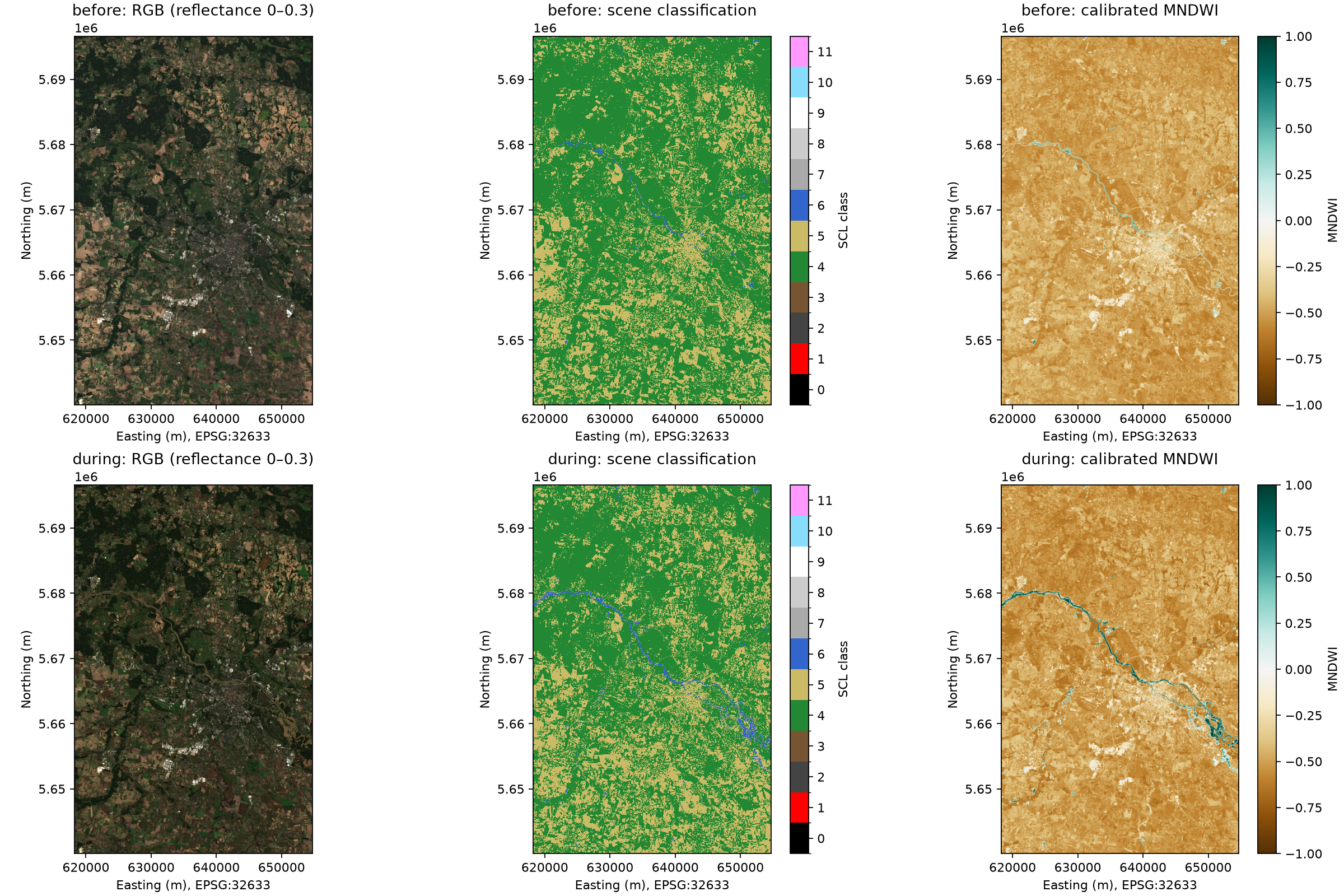
Top row: 6 September 2024, labelled before. Bottom row: 21 September 2024, labelled during. The RGB display stretch is identical on both dates. SCL classes 4, 5 and 6 denote vegetation, non-vegetated land and water.
The later scene shows a stronger water signal and wider water-like patches along the main river corridor. The change map concentrates the largest increases there, with smaller scattered changes elsewhere. These patterns support using the pair for a worked surface-water comparison.
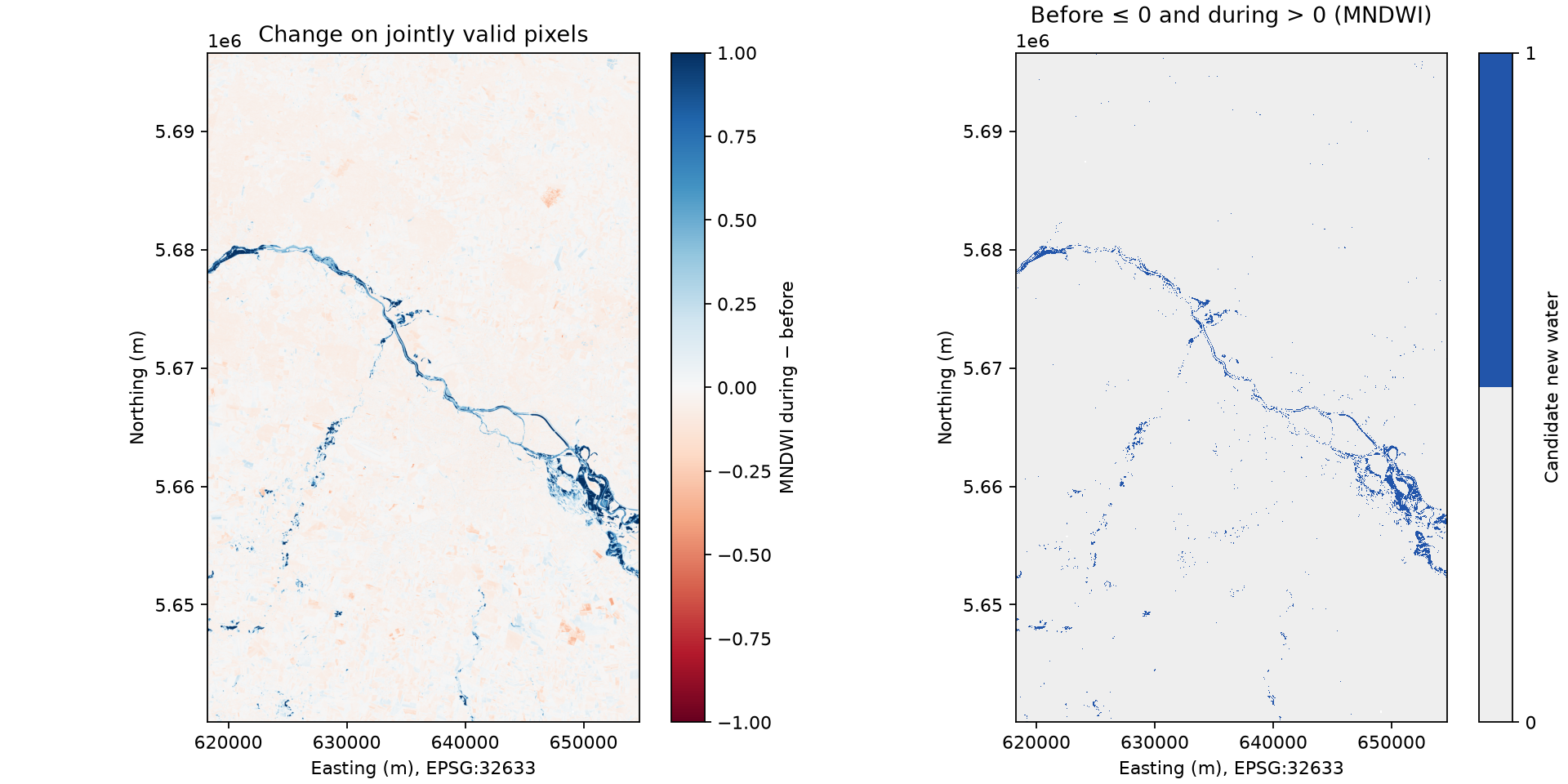
Left: MNDWI on 21 September minus MNDWI on 6 September. Right: pixels changing from MNDWI at most zero to a positive value. Only pixels valid on both dates are compared.
In the SCL layer from the later scene, 36,119 of the 64,112 candidate pixels are labelled as water, 27,893 as non-vegetated land and 100 as vegetation. Thus about 44% are not labelled as water by SCL. Wet soil, mixed pixels and changes unrelated to inundation may contribute; SCL itself is not independent ground truth. Do not describe every candidate pixel as confirmed flooding.
What to do next
These articles explain how to access EODATA through a mounted filesystem:
To use /eodata on an NSIS Cloud VM, follow How to create new Linux VM in OpenStack Dashboard Horizon on NSIS Cloud and connect it to the eodata network. Automatic and manual mounting are covered in How to mount eodata using s3fs in Linux on NSIS Cloud.
For an alternative mounting tool, follow How to mount EODATA as a filesystem using Goofys in Linux on NSIS Cloud.
EODATA credentials are separate from the keys for your own Object Storage buckets. Obtain them by following Obtain S3 credentials for EODATA Access from NSIS Cloud Dashboard.